Project write-up · Data engineering · PostgreSQL 18
What 22 Million Sensor Readings Taught Me About Postgres
A robot drove around a campus 27 times over 15 months. I loaded everything it recorded into a database with only 512 MB of memory, then tried to make it fast. Here's what worked, what didn't, and what surprised me.
By Raine Kyro VisayaNovember 2026About a 14-minute read
- 21.9M
- rows of sensor data
- 27
- drives, Jan 2012 – Apr 2013
- 512 MB
- memory for Postgres
- 113×
- faster time-window queries
Intro
Why a robot, and why Postgres
This semester I'm taking CS 421, and in class we work with MySQL. The more we covered how a database stores and finds data, the more I wanted to go deeper than an assignment allows. So I picked a different open-source database, PostgreSQL, because it has features I wanted to try for myself: several index types, detailed query plans, and PostGIS for maps.
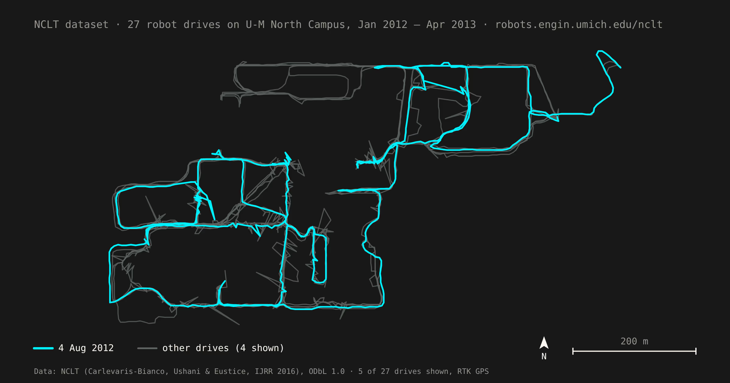
I also like robotics, so I went looking for real robot data and found the NCLT dataset from the University of Michigan. Between January 2012 and April 2013, a Segway robot drove around Michigan's North Campus 27 times. It drove in every season, through snow and summer leaves and past construction, and it recorded everything: wheel motion, an inertial sensor, a regular GPS and a high-accuracy RTK GPS.
Here's the scale. Five sensor streams, recording between 2.5 and 108 times per second, add up to 21.9 million rows: 14.1M odometry rows, 6.2M from the inertial sensor (IMU), 954K regular GPS fixes and 653K RTK GPS rows. That's far bigger than anything in my assignments.
Then I added one rule to make it interesting: Postgres 18 runs in a Docker container capped at 512 MB of memory, with 128 MB for its own cache. The odometry table alone is 1.22 GiB, so most of the data can't sit in memory. I wanted to see what happens when data outgrows RAM, because that's when database design starts to matter.
But before I could make anything fast, I had to get 22 million rows in without ever leaving a half-loaded session behind.
Phase 1
Getting the data in safely
Loading a session takes a few seconds, and a lot can go wrong in a few seconds. The laptop sleeps, the container runs out of memory, I press Ctrl+C. If the loader dies halfway, some tables have the new session and some don't. Every query after that quietly gives wrong answers, and nothing warns you.
So the loader works in two steps. First, it streams each CSV file into a scratch staging table and checks that the row count matches the number of lines in the file. Then it swaps the staging data into the real tables. All of that happens inside one transaction, so either the whole session lands or none of it does.
Act 1 · Loading
The loading pipeline
Everything inside the dashed box is one transaction. The red marks show where I crashed it on purpose.
The swap itself is short. For each sensor table it deletes the session's old rows and inserts the new ones from staging:
BEGIN;
-- for each of the 5 sensor tables:
DELETE FROM odometry WHERE session_id = 17;
INSERT INTO odometry (session_id, utime, x, y, z, roll, pitch, heading)
SELECT 17, utime, x, y, z, roll, pitch, heading FROM staging_odometry;
-- ...then record the session in dim_session
COMMIT;  -- nothing is visible until this line
A design like this is only believable if you try to break it. I added
a crash hook, an environment variable called NCLT_CRASH_AT, that kills the process instantly at a chosen point: during the
first COPY, during the last COPY, or in the middle of the swap. I tested each point twice, on an
empty database and while reloading a session that was already there.
That's 6 crashes, and every one left the tables exactly as they
were before.
Why COPY instead of INSERT
The Postgres docs recommend COPY for bulk loading,
and I wanted to see how much it matters. With row-by-row INSERT, every row is its own statement: Postgres parses it, plans it, runs
it and replies, 270,000 times for one IMU file. COPY sends the whole file as one stream that the server reads directly.
Act 1 · Loading
COPY loads 21× faster than row-by-row inserts
One IMU file (269,979 rows), median of 3 runs
Across the 26 sessions I loaded in one go, the actual loading took 104
seconds, about 200,000 rows per second end to end. Downloading the
archives took most of the 5.5 minutes. For a whole session file,
COPY wins every time. Batched inserts still make
sense for a trickle of new rows arriving one at a time, which isn't this
project.
What if two readings have the same timestamp?
Real sensors can log the same timestamp twice. My first idea was to average the two readings. Then I realized an average describes a position the robot was never actually in: a ghost reading. So the rule is last row wins. The later line in the file replaces the earlier one, and the loader counts every row it drops. In my data that count has been zero so far, but the rule and its test are there for the day it isn't.
Phase 2
Listening to the data
Before optimizing anything, I needed to know what "normal" looks like. My plan was to catalog every time a sensor went quiet, a dropout. But what counts as quiet? A sensor that reports every 20 ms isn't broken after 30 ms of silence.
Instead of guessing, I measured the gap between consecutive readings for every sensor in all 27 sessions. Then I set each threshold just above that sensor's normal pauses:
| Sensor | Normal pauses (p99) | Longest pause | Dropout if quiet for |
|---|---|---|---|
| IMU | 41–51 ms | 100 ms | 0.15 s |
| Odometry | 20–21 ms | 75 ms | 0.05 s |
| GPS | 0.27–0.60 s | 739 s | 2 s |
| RTK GPS | 1.0–1.9 s | 4.07 s | 5 s |
Only one sensor really drops out: the regular GPS. Across 26 of the 27 drives it went silent 88 times, for 3 hours in total. A typical drive loses about 8% of its GPS time.
Act 2 · Listening to the data
The regular GPS loses about 8% of a typical drive
Share of each session with no GPS fix for more than 2 s, all 27 sessions
The RTK receiver never stops talking
I expected the RTK GPS to drop out too. It never went quiet for more than 4.07 seconds in any session. During the 634-second GPS outage on 4 August 2012, it kept reporting: 919 readings. About half of those were weaker 2D fixes with an average error of 37 metres. So the RTK receiver's outages don't show up as silence. They show up as worse accuracy, and that's how I track them.
The robot that visited the Gulf of Guinea
When I first added map coordinates with PostGIS, the whole step
crashed with
Point outside of projection domain. One RTK
reading, out of 326,000, sat at latitude 0, longitude 0. That spot is
in the ocean off West Africa, and mapping people call it "Null
Island". The receiver had labeled that reading a full 3D fix, and its
own error estimate was 6,356,586 metres. That's close to the radius of
the Earth, which suggests the receiver sent an empty position.
The readings 2 seconds before and 3 seconds after were right where they should be, on campus. So it was a single glitch, and the fix was a rule: a reading gets a map position only if its fix mode is at least 2D and it isn't at (0, 0).
ALTER TABLE gps_rtk ADD COLUMN geom geometry(Point, 32617)
  GENERATED ALWAYS AS (
    CASE WHEN mode >= 2 AND lat <> 0 AND lng <> 0
         THEN ST_Transform(ST_SetSRID(ST_MakePoint(degrees(lng), degrees(lat)), 4326), 32617)
    END   -- anything else gets no position (NULL)
  ) STORED;
The lesson I took from it: don't fully trust a quality flag that the device sets about itself.
One more thing I noticed: partway through the year, the IMU's timing got slightly noisier and the RTK receiver started reporting more often. It looks like someone changed a setting on the robot. My thresholds sit above both behaviors.
Now that I trusted the data, it was time to make it fast.
Phase 3
Making queries fast
The first query I optimized is the most common question you'd ask this data: give me one session's IMU readings between two timestamps. The answer is 2,825 rows out of 6.2 million.
With no index, Postgres has no way to find those rows except to read the whole table, all 88,459 pages (691 MiB), and throw away almost everything. That took 1.05 seconds at p95. The query plan says it plainly:
Before: no index
Gather
  -> Parallel Seq Scan on imu
Buffers: shared read=88459
Execution Time: 791.6 ms
After: B-tree on (session_id, utime)
Index Scan using imu_pkey on imu
Buffers: shared hit=3 read=54
Execution Time: 0.7 ms
The fix was a B-tree index on (session_id, utime). Postgres can now jump straight to the right session and read just
the slice of time it needs: 54 pages instead of 88,459, and 9.3 ms at p95. That's 113× faster. (These two
plans are abridged from my saved results; each is one cold run.)
The column order matters. It works like a phone book sorted by last
name, then first name. The equality filter (session_id = 17) goes first, so Postgres can jump straight to that session's
section. The range filter (utime BETWEEN …)
goes second, so the matching rows sit next to each other inside it.
The 48 KiB index
Postgres also has a much smaller index type called BRIN. Instead of pointing to every row, it stores just the smallest and largest timestamp for each block of 128 pages. My loader writes rows in time order, so each block covers a short, tidy slice of time, and BRIN can skip almost every block.
Act 3 · Making queries fast
A 48 KiB index came within 1.5× of a 186 MiB one, until I shuffled the rows
Time-window query, cold cache, 30 runs each, log scale
The BRIN index is 48 KiB. The B-tree is 186 MiB, about 4,000 times bigger, and BRIN's median was only 1.5× slower. Then I tried to break it: I made a copy of the same rows in random order. Now every block holds readings from every session and every month, so BRIN can't skip anything. The query went to 283 ms at p95, about as slow as having no index at all.
So BRIN is a great deal, but only while the data stays in time order. In this project, the loader is what keeps that promise.
One Postgres 18 bonus: a query that filtered on time alone, with no
session, could still use the
(session_id, utime) index thanks to a new feature
called skip scan. It ran in 8.2 ms. Older versions of
Postgres couldn't use a B-tree when its first column had no filter.
Phase 4
When indexes are the wrong tool
Indexes help when a query needs a small piece of a big table. But some questions need the whole table, and for those no index can help. What helped was changing the question.
The 24-second report
"Distance, duration and top speed for each session" sounds simple, and the answer is only 27 rows. But to compute it, Postgres has to read all 14.1 million odometry rows, sort them by time, and compare each one with the previous one. The sort didn't fit in memory, so it spilled 1.66 GiB to disk. The query took 24 seconds at p95.
The answer only changes when a new session is loaded. So I computed it once, in about 20 seconds, and stored the 27 rows in a small summary table. Reading it takes 1.3 milliseconds. The catch is that the summary goes stale if I forget to refresh it, so the next version of the loader will update it in the same transaction as each new session.
The index that made things slower
Next question: "the last 100 IMU readings of every session." The obvious SQL numbers every row in each session and keeps the first 100:
Before: number everything, keep 2,700 rows
SELECT *
FROM (
  SELECT imu.*, row_number() OVER (
           PARTITION BY session_id
           ORDER BY utime DESC) AS rn
  FROM imu
) ranked
WHERE rn <= 100;
After: ask each session for its newest 100
SELECT i.*
FROM dim_session s
CROSS JOIN LATERAL (
  SELECT *
  FROM imu
  WHERE imu.session_id = s.session_id
  ORDER BY utime DESC
  LIMIT 100
) i;
The first version took 7.3 seconds at p95. Adding the B-tree made it slower: its median went from 2.05 s to 2.25 s, because Postgres still numbered all 6.2 million rows, now reading the index and the table. The rewrite asks the question the index can actually answer: for each of the 27 sessions, walk backwards from the newest reading and stop after 100. It reads 128 pages instead of 88,459, and takes 10 ms at p95.
The same idea worked on the map data. A per-cell RTK error report went from 250 ms to 3 ms once I stored its answer in a materialized view.
If I had to put this Phase in one sentence: an index only helps when the query lets the database stop early.
Act 4 · The whole picture
Every query got faster, from 2.1× to ≈18,000×
p95 latency before → after, cold cache, log scale
Phase 5
The surprises
I tested each change on its own first, then combined the winners into one final setup. Not everything behaved the way I expected.
The planner changed its mind
One query found RTK readings with large errors. Tested alone with its indexes, it took 8 ms, using quick index lookups. In the final combined setup, with indexes that did the same job, Postgres chose a completely different strategy: it read the whole RTK table and built a hash table. It took 30 ms.
The indexes didn't change. What changed was the planner's decision. My best guess is that the final setup refreshed the table statistics, and the new numbers tipped the planner's cost estimate the other way. I'm still testing that. Either way, it taught me to always measure the combination, not just the parts.
"Warm" wasn't warm
I expected warm runs, with the cache already loaded, to be much faster than cold ones. For the full-table queries, they weren't. Even on a warm run, the no-index time-window query still had to fetch 87,895 of its 88,459 pages from outside Postgres's cache. A 691 MiB table simply doesn't fit in 128 MB. Only queries with small working sets, like index lookups, really benefit from a warm cache. That's why every headline number in this post is a cold one.
What's next
What breaks at 10×
The data stops at 27 drives, but real fleets don't. Here's what I think would break if the data grew ten times, to about 220 million rows, with the same 512 MB. These are estimates from my numbers, not measurements.
| Today | At 10× (estimate) | What I'd change |
|---|---|---|
| All indexes together: 704 MiB | About 7 GiB, so almost none of it stays in memory | Split tables by session or month, and use tiny BRIN indexes on old data that never changes |
| Loading: 104 s | About 17 minutes | Load sessions in parallel, each in its own transaction |
| Summary table rebuild: 20 s | About 3 minutes | Update each session's summary row as part of loading it |
| All analysis runs in Postgres | Big scans compete with quick lookups | Export to Parquet files and run the heavy analysis in DuckDB |
The end
What I learned
- Count pages, not just milliseconds. The number of pages a query reads explained almost every result in this project. Milliseconds tell you something changed; pages tell you why.
- A tight memory limit keeps you honest. With 512 MB, I couldn't hide a bad query behind a big cache.
- Understanding the data was half the work. Thresholds, a mid-year settings change, and a robot that briefly claimed to be in the ocean all had to be handled before any number could be trusted.
- The biggest wins came from better questions. Indexes gave 2× to 113×. Rewrites and stored answers gave 83× to about 18,000×.
- Optimizations interact. A change that wins on its own can lose in combination, so measure the whole setup.
The 24-second question now takes 1.3 milliseconds. Postgres didn't get faster. I just stopped asking it to read 14 million rows to count to 27.